It stands to reason that the first post on a blog should be a statement about the planned content of said blog.
Eh-hem…
This is my personal blog where I’ll house whatever stupid / interesting crap comes into my head. I expect the content here will mostly cover math / graphs, though if I have something to say about a piece of media, don’t be surprised if it shows up here.
So… that’s the general overview.
More specifically, I’d like to talk about a few of the concepts that’ve been on my mind lately. A few months back I attempted to do this in video. I wrote three scripts, recorded audio and visual aid, and one video came out. Evidently videos just aren’t my medium as the one video had terrible visuals and the other two never got finished because I have no drive to actually edit anything.
This, of course, is what brings us here. I’d like my inaugural post to start with a sort of memorial for the videos that never came to be. As such, the remainder of this post shall be the leftover scripts to those videos and whatever interjections I have to make.
Script in normal, comments in [bold], here we go…
The Spin Smile Analysis:
I think there are two reasons why it’s a shame that the graph Spin smile no longer appears under any staff picks lists on the desmos homepage. The first reason is that we’ll never know who made it, and the second is that it shows a better understanding of multivariable functions I see in most graph art.
The graph itself consists of one massive equation and 6 variables that are there to control, respectively, the current angle, the size and position of the eyes, and the size of the mouth and head. Most striking among these is probably the fact that the equation itself is only one equation. It’s got unshaded regions like the eyes and mouth, but it doesn’t use domain restrictions to do this. So how does it do it?
This method of graphing multiple shapes has to do with the fact that any number multiplied by zero is zero, but before we talk about that we have to discuss multivariable functions. Let’s back up a bit. In mathematics the single variable functions we tend to use are simply rules for taking input numbers and outputting other numbers. For instance, the function f(x)=x^2 takes the input “x” and outputs that number multiplied by itself. Typically these functions are represented by having each value of the inputs correspond to some point on a number line. Then, to visualize the function we draw a curve above and below the number line such that at any position, the distance between the curve and the number line is equal to the output of the function at that point.
Now, you probably could’ve figured that out, but it’s worth going over a specific case before we go and generalize it. So what’s a multivariable function? Simple, it’s a function that takes two input numbers and outputs one number. For instance, the multivariable f(x,y)=x+y would take the inputs “x” and “y” and output their sum. Given the generally accepted curve method for single variable functions, one’s first intuition for visualizing multivariables may be to use points along a plane as the inputs, then map those to some curved surface in 3D space. This is technically possible in desmos, if you use a pre-built graph such as this one [would have shown this on screen] like they seem to suggest,[would have shown this on screen] but for this graph, we only need to visualize the points that are positive, negative, and equal to zero.
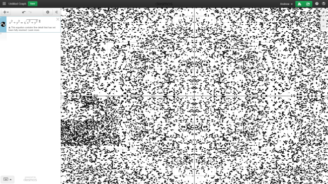
If you define some multivariable function in desmos, say this equation [for visual, paste into Desmos: f\left(x,y\right)=\sqrt{x^2+y^2}] for the distance to zero, you can then set it equal to some number and desmos will graph a curve that represents every point where the output of the function is equal to said number. The distance equation can be set equal to something like 2, and it will graph a circle with a radius 2. It can also be set as an inequality, like less than 2, and it will shade the region where the condition is still met.
All that said, the real magic happens when one takes two multivariables and sets them equal to zero. Here [paste into Desmos: f\left(x,y\right)=x^2+y^2-1 and g\left(x,y\right)=\left(x-h\right)^2+\left(y-k\right)^2-1] I have defined two multivariable functions. If I set either equal to zero, one will graph a circle of radius one, the other will graph the same around some arbitrary point of my choosing, likewise setting either to less than zero will shade said circle’s interior. So what happens when I multiply them together and set that equal to zero? Well, the answer is simple if you consider what’s happening when I graph either equation on it’s own. The circle appears at the points when the function is equal to zero, and can be shaded at the points when it’s negative. Since any number times zero is zero, the multiplied functions will be equal to zero at any point where either is zero. Therefore, we can deduce that the multiplied graph should show both circles and, sure enough, it does! [paste into Desmos: f\left(x,y\right)g\left(x,y\right)\le 0] Likewise, by overlapping the circles, the shading will invert, which makes sense given that, you know, a negative times a negative equals a positive. [would have cut to the clip from Stand and Deliver for this line] The multiplication method can be used to graph any set of functions simultaneously, but we should get back to Spin smile.
Here [for visual, look here] I have broken Spin smile down to all its constituent functions. Looking at them, a pattern seems to emerge, all the instances of t seem to be in little modules of x, y, and a trig function involving t as a rotation variable. These little modules are a little something I’ve been calling the function spinner, perhaps more aptly called a rotation transformation or something. The idea is that you take the function you want to rotate and replace, say, every “x” with a “cos(t)x-sin(t)y)” and every “y” with a “cos(t)y+sin(t)x)”. Suffice it to say that these little transformations can be used to rotate any graph, whether it be multivariable or parametric. [paste into Desmos: \left(\cos \left(a\right)X\left(t\right)-\sin \left(a\right)Y\left(t\right),\cos \left(a\right)Y\left(t\right)+\sin \left(a\right)X\left(t\right)\right)]
I could separate out all the rotation transformations, but for the purposes of this analysis, I think it makes more sense to just set the angle to zero and simplify. [for visual, look here] From here it’s plain to see that it’s just simple circles for the eyes and head, and the relative strangeness going on here is the mouth.
After all I’ve said, the half circle for the mouth is the thing on this graph that I see as it’s crowning achievement. I’ve been trying to figure out a way to graph half circles for months, and here comes an elegant solution gift wrapped in a silly face. Looking at the mouth individually, we can see that it’s composed of three equations, marked here [for visual, look here] as one, two, and three. One is an equation for this [paste into Desmos: 0\ge \left(x\cdot \frac{\left|y\right|-y}{2y}\right)^2+y^2-b^2] strange band with a half circle coming off of it. Two and three just graph the band and are there to cancel it out, in much the same way that the circles canceled out earlier. Two and three are just lines, the real meat is in equation number one.
So how does it work? Looking at it, it just looks like a messed up equation for a circle, with “b” as the radius and something odd going on in the “x” compartment. The secret lies there. The fraction [paste into Desmos: \left(x\cdot \frac{\left|y\right|-y}{2y}\right)] that’s rooming with x simplifies to look like this. [paste into Desmos: \left(x\frac{1}{2}\left(\frac{\left|y\right|}{y}-1\right)\right)] Looking at that y bit as a function of x reveals that it simply outputs one or negative one based on whether the input is positive or negative, respectively. In context, that would mean it’s positive at every point above the origin vertically and negative at every point below. That means that above the origin it’s basically graphing this [paste into Desmos: 0\ge y^2-b^2] function, which accounts for the band, and below the origin it’s graphing this [paste into Desmos: 0\ge x^2+y^2-b^2] function, which accounts for the half circle. An elegant method for getting a half circle, if I do say so myself.
Add in the rest of the mouth equations to cancel the rest of the half circle, replace the rest of the face, and swap all x’s and y’s with spinners, and you’ve got Spin smile. I really like it. It does a lot with the tools desmos provides and a good understanding of mathematics. It’ll probably never make it onto the creative art staff picks as it’s neither high detail or a dirty trace, but I think it still stands as a showcase of what’s possible in desmos graph art. And with the level of stuff everyone seems so fond of making, I like it for it’s clever problem solving. I guess you could say it makes me smile.
The Boat Guy Analysis: [This one has so many visual notes that I’ll adress them later]
I’ve been making graph art for about four months now. I’ve made some good stuff and some bad stuff. I bet it all started with this graph.
Imagine it, March of 2015, I’m casually looking through one of desmos’ staff picks lists and I find this piece of graph art, a guy rowing on a boat in an endless sea; the sun is in the sky and some clouds are passing by. The intricacy of everything is astounding and even more… it moves! My younger self is impressed and saves the graph, renaming the save in the process. “I found this boat guy”. great
I don’t really like how I went about this, making bloated lists of all the cool stuff is the real way to go, but I digress.
This nameless graph was the first thing I thought of when I sat down with a computer and decided to make some dumb fish. It’s focus on shape and animation is probably the best part. Let’s take this thing apart.
Simple parts first. The sun is just a couple of circles and there’s this green… thing under the water. Easy, next. The water is pretty clearly made of some sine waves, though in these we can see the emphasis on shape come through. It’s three layers to create a sense of shading and depth. Looking at the individual layers, we can see that each is made from taking two sine waves and adding them together to create this lumpy, inconsistant look. The lumps on each of each of these are all formed by the same sine, which has a low amplitude and a short wavelength since it’s just there to add detail. The rest of the waves are all different. Between them, x and s are multiplied by varying values so they won’t line up or move together, respectively. Capping them off, the purple wave is at a lower height so that it gives depth to the water and doesn’t stand out as, well, purple.
Moving on to the figure himself we’ll notice the equations becoming a lot heavier in length. The boat, for example is this long thing. Now it didn’t need to be that long, for instance this component that’s seen twice could’ve been easily shortened to look like this. Not sure why it’s left long, but what’s more important is it’s purpose. The whole thing is multiplied by an x to the half power which, when moving the slider s, rocks the whole boat. Since it’s on both sides of the inequality, the boat moves with uniformity, never changing it’s shape all that much. The last unaddressed component of the boat is this bit modified from the equation for an ellipse that gives the lower part of the boat it’s round shape.
The person in the boat revisits most of the same ideas. The head is just a circle with the component that rocked the boat to keep it moving naturally. For that matter, I’ve highlighted here the instances of this bit throughout the figure. The body is just more of the same, this square root bit defines it’s overall shape, while the afore highlighted bit keeps it moving. Desmos will graph any function that’s just in terms of x as if it were equal to y, so the only thing left is this other root that get’s added in and then immediately subtracted. On it’s own it looks like a strange thing to do until you realize that desmos can’t handle imaginary numbers. I did a similar thing with my fish graph: the idea is that since desmos has no definition for any square roots of negative numbers, it will just not graph any regions of equations that would require them, even if they’re divided by themselves or subtracted from themselves. The result is that one can stop any line freely without having to use desmos’ range phrasing, which is exactly what this graph does. Without these stopping the curve, the boat guy’s body would explode out to the left and look bad. Why they didn’t just use a range restriction is anyone’s guess, but I suspect it’s probably the same reason that all the shapes’ borders are left hashed.
The last part of the figure is the rowing oar line, which is by far the longest equation in this graph. However, I think you’ll find that it doesn’t look quite as long when I highlight how much of this thing is just there to cut off the line. Both cutoffs have two components, such that the line is stopped with a minimum and a maximum, with one stopping it’s horizontal distance and one stopping it’s vertical. Aside from the cutoffs, the rest is pretty straight forward. It’s just a line. The most interesting part is probably the fact that it creates the rotating motion with use of a sine function. You see, based on the value of s, this sine will alternate between values of 1 and -1. When it’s 1, the x’s cancel and it’s just a horizontal line with a height of .4. When it’s -1, the x’s will add and it’ll be a line with a slope of 2 and an x intercept at the average of these two numbers, 6.8. The transition between these two states coupled with the rocking component is what gives the oar it’s fluidity. Now onto the last part.
The clouds. First thing to note about them is that there’re two of them, which can be seen in the equation itself. In my Spin smile video I talked about how multiplying together multivariable equations can allow one to graph as many things at the same time as they so choose. That’s exactly what’s going on here. Looking at the components of the equation, the only differences between the actual clouds have to do with position and movement. Other than that, the clouds’ equations just look like ellipsoids, except for the key difference: the sin under x. Ordinarily this would be a constant that stood for the width of the ellipse. Since it’s a function based on y, the width will change according to y’s value. This can be clearly seen if we put a graph of the sine over the cloud. Sure enough, when the sine of 10 y equals 0, so to does the width of the cloud.
Now, when looking at the cloud up close, you can see exactly what’s going on with it. It just looks like this stack of ovals, which, given the way it’s constructed, is what it is, but what I think is really important to note about this graph is how it looks when you zoom out. The borders between the individual segments disappear into each other as desmos becomes incapable of dealing with the amount of detail it would take to determine the shape of each. However, this works greatly in the graph maker’s favor as it fills out the clouds, making them look more like solid things than stacks of segments.
And that’s what this graph really has going for it. It pays great attention to the way that desmos handles multivariable equations and uses it to it’s advantage in handling the shape of these clouds. Likewise, it’s aware of the shaping of the boat and figure at all times, keeping them looking right, and of the water, giving it depth and an organic lumpiness that is characteristic of water. The graph maintains its emphasis on quality shapes when set in motion, keeping everything looking right and organic for the scene. It’s this kind of attention to detailed form and motion that puts it above so much other graph art, and it’s this that makes it such an inspiration to behold even after all this time.
Shine on you crazy graphman.
Alright, now that the text of those is posted. Great.
After having gone a few months without editing these videos, a friend approached me saying that he’d be willing to edit any math videos I wanted to make. We discussed a bit and I sent him all of my production files on google docs so that he could get editing at his leisure. However, that was a month and a half ago and I’m not getting a sense that he’ll ever get around to those things. Maybe what I had recorded is so ugly that he doesn’t want to look at it, maybe the fact that some of the visuals don’t have files already prepared was off-putting. Either way, the fact of the matter is that I want to talk about other things, and those are somewhat dependent on these two videos being in some canon of mine, so I needed to release them somehow. Thus, blog.
If you’re also insane enough to want to attempt editing these things for me, you can find the files here.